Tree Based Methods

class: center, middle, inverse, title-slide

# Tree Based Methods
## IS382 - Predictive Modeling
### Jason Bryer
### Week 7

---
# Classification and Regression Trees

The goal of CART methods is to find best predictor in X of some outcome, y. CART methods do this recursively using the following procedures:

* Find the best predictor in X for y.
* Split the data into two based upon that predictor.
* Repeat 1 and 2 with the split data sets until a stopping criteria has been reached.

There are a number of possible stopping criteria including: Only one data point remains.

* All data points have the same outcome value.
* No predictor can be found that sufficiently splits the data.

---
# Recursive Partitioning Logic of CART

.pull-left[
Consider the scatter plot to the right with the following characteristics:

* Binary outcome, G, coded “A” or “B”.
* Two predictors, x and z
* The vertical line at z = 3 creates the first partition.
* The double horizontal line at x = -4 creates the second partition.
* The triple horizontal line at x = 6 creates the third partition.
]
.pull-right[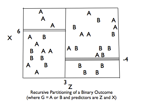
![](images/Partitioning.png)
]

---
# Tree Structure

.pull-left[
* The root node contains the full data set.
* The data are split into two mutually exclusive pieces. Cases where x > ci go to the right, cases where x <= ci go to the left.
* Those that go to the left reach a terminal node.
* Those on the right are split into two mutually exclusive pieces. Cases where z > c2 go to the right and terminal node 3; cases where z <= c2 go to the left and terminal node 2.
]
.pull-right[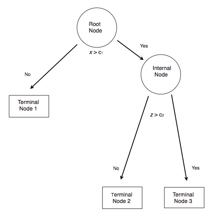
![](images/TreeDiagram.png)
]

---
# Sum of Squared Errors

The sum of squared errors for a tree *T* is:

`$$S=\sum _{ c\in leaves(T) }^{  }{ \sum _{ i\in c }^{  }{ { (y-{ m }_{ c }) }^{ 2 } }  }$$`

Where, `${ m }_{ c }=\frac { 1 }{ n } \sum _{ i\in c }^{  }{ { y }_{ i } }$`, the prediction for leaf \textit{c}.

Or, alternatively written as:

`$$S=\sum _{ c\in leaves(T) }^{  }{ { n }_{ c }{ V }_{ c } }$$`

Where `$V_{c}$` is the within-leave variance of leaf \textit{c}.

Our goal then is to find splits that minimize S.

---
# Advantages of CART Methods

* Making predictions is fast.

* It is easy to understand what variables are important in making predictions.

* Trees can be grown with data containing missingness. For rows where we cannot reach a leaf node, we can still make a prediction by averaging the leaves in the sub-tree we do reach.

* The resulting model will inherently include interaction effects. There are many reliable algorithms available.

---
# Regression Trees

In this example we will predict the median California house price from the house’s longitude and latitude.

``` r
str(calif)
```

```
## 'data.frame':	20640 obs. of  10 variables:
##  $ MedianHouseValue: num  452600 358500 352100 341300 342200 ...
##  $ MedianIncome    : num  8.33 8.3 7.26 5.64 3.85 ...
##  $ MedianHouseAge  : num  41 21 52 52 52 52 52 52 42 52 ...
##  $ TotalRooms      : num  880 7099 1467 1274 1627 ...
##  $ TotalBedrooms   : num  129 1106 190 235 280 ...
##  $ Population      : num  322 2401 496 558 565 ...
##  $ Households      : num  126 1138 177 219 259 ...
##  $ Latitude        : num  37.9 37.9 37.9 37.9 37.9 ...
##  $ Longitude       : num  -122 -122 -122 -122 -122 ...
##  $ cut.prices      : Factor w/ 4 levels "[1.5e+04,1.2e+05]",..: 4 4 4 4 4 4 4 3 3 3 ...
```

---
# Tree 1

``` r
treefit <- tree(log(MedianHouseValue) ~ Longitude + Latitude, data=calif)
plot(treefit); text(treefit, cex=0.75)
```

---
# Tree 1

---
# Tree 1

``` r
summary(treefit)
```

```
## 
## Regression tree:
## tree(formula = log(MedianHouseValue) ~ Longitude + Latitude, 
##     data = calif)
## Number of terminal nodes:  12 
## Residual mean deviance:  0.1662 = 3429 / 20630 
## Distribution of residuals:
##     Min.  1st Qu.   Median     Mean  3rd Qu.     Max. 
## -2.75900 -0.26080 -0.01359  0.00000  0.26310  1.84100
```

Here “deviance” is the mean squared error, or root-mean-square error of `$\sqrt{.166} =  0.41$`.

---
# Tree 2, Reduce Minimum Deviance

We can increase the fit but changing the stopping criteria with the mindev parameter.

``` r
treefit2 <- tree(log(MedianHouseValue) ~ Longitude + Latitude, data=calif, mindev=.001)
summary(treefit2)
```

```
## 
## Regression tree:
## tree(formula = log(MedianHouseValue) ~ Longitude + Latitude, 
##     data = calif, mindev = 0.001)
## Number of terminal nodes:  68 
## Residual mean deviance:  0.1052 = 2164 / 20570 
## Distribution of residuals:
##     Min.  1st Qu.   Median     Mean  3rd Qu.     Max. 
## -2.94700 -0.19790 -0.01872  0.00000  0.19970  1.60600
```

With the larger tree we now have a root-mean-square error of 0.32.

---
# Tree 2, Reduce Minimum Deviance

---
# Tree 3, Include All Variables

However, we can get a better fitting model by including the other variables.

``` r
treefit3 <- tree(log(MedianHouseValue) ~ ., data=calif)
summary(treefit3)
```

```
## 
## Regression tree:
## tree(formula = log(MedianHouseValue) ~ ., data = calif)
## Variables actually used in tree construction:
## [1] "cut.prices"
## Number of terminal nodes:  4 
## Residual mean deviance:  0.03608 = 744.5 / 20640 
## Distribution of residuals:
##      Min.   1st Qu.    Median      Mean   3rd Qu.      Max. 
## -1.718000 -0.127300  0.009245  0.000000  0.130000  0.358600
```

With all the available variables, the root-mean-square error is 0.11.

---
# Classification Trees

Predicting who survived the Titanic.

* `pclass`: Passenger class (1 = 1st; 2 = 2nd; 3 = 3rd)
* `survival`: A Boolean indicating whether the passenger survived or not (0 = No; 1 = Yes); this is our target
* `name`: A field rich in information as it contains title and family names
* `sex`: male/female
* `age`: Age, a significant portion of values are missing
* `sibsp`: Number of siblings/spouses aboard
* `parch`: Number of parents/children aboard
* `ticket`: Ticket number.
* `fare`: Passenger fare (British Pound).
* `cabin`: Does the location of the cabin influence chances of survival?
* `embarked`: Port of embarkation (C = Cherbourg; Q = Queenstown; S = Southampton)
* `boat`: Lifeboat, many missing values
* `body`: Body Identification Number
* `home.dest`: Home/destination

---
# Classification using `rpart`

``` r
(titanic.rpart <- rpart(survived ~ pclass + sex + age + sibsp,
   data=titanic.train))
```

```
## n= 981 
## 
## node), split, n, deviance, yval
##       * denotes terminal node
## 
##  1) root 981 231.6514000 0.3822630  
##    2) sex=male 640  98.7437500 0.1906250  
##      4) pclass>=1.5 497  62.2776700 0.1468813  
##        8) age>=4.5 460  52.1739100 0.1304348 *
##        9) age< 4.5 37   8.4324320 0.3513514  
##         18) pclass>=2.5 28   4.1071430 0.1785714 *
##         19) pclass< 2.5 9   0.8888889 0.8888889 *
##      5) pclass< 1.5 143  32.2097900 0.3426573 *
##    3) sex=female 341  65.2903200 0.7419355  
##      6) pclass>=2.5 157  39.2101900 0.5159236 *
##      7) pclass< 2.5 184  11.2173900 0.9347826 *
```

---
# Classification using `rpart`

``` r
plot(titanic.rpart); text(titanic.rpart, use.n=TRUE, cex=1)
```

---
# Classification using `ctree`

``` r
(titanic.ctree <- ctree(survived ~ pclass + sex + age + sibsp, data=titanic.train))
```

```
## 
## 	 Conditional inference tree with 9 terminal nodes
## 
## Response:  survived 
## Inputs:  pclass, sex, age, sibsp 
## Number of observations:  981 
## 
## 1) sex == {female}; criterion = 1, statistic = 286.055
##   2) pclass <= 2; criterion = 1, statistic = 75.735
##     3) pclass <= 1; criterion = 0.989, statistic = 9.029
##       4)*  weights = 107 
##     3) pclass > 1
##       5)*  weights = 77 
##   2) pclass > 2
##     6) sibsp <= 2; criterion = 0.99, statistic = 9.086
##       7)*  weights = 143 
##     6) sibsp > 2
##       8)*  weights = 14 
## 1) sex == {male}
##   9) pclass <= 1; criterion = 1, statistic = 22.494
##     10) age <= 36; criterion = 0.991, statistic = 9.236
##       11)*  weights = 45 
##     10) age > 36
##       12)*  weights = 98 
##   9) pclass > 1
##     13) age <= 4; criterion = 0.993, statistic = 9.853
##       14) pclass <= 2; criterion = 0.999, statistic = 14.671
##         15)*  weights = 9 
##       14) pclass > 2
##         16)*  weights = 28 
##     13) age > 4
##       17)*  weights = 460
```

---
# Classification using `ctree`

``` r
plot(titanic.ctree)
```

---
# Model Performance

The use of statistical models to predict outcomes, typically on new data, is called predictive modeling. Logistic regression is a common statistical procedure used for prediction. We will utilize a **confusion matrix** to evaluate accuracy of the predictions.

---
class: font80
# Predicting Heart Attacks

Source: https://www.kaggle.com/datasets/imnikhilanand/heart-attack-prediction?select=data.csv

``` r
heart <- read.csv('../course_data/heart_attack_predictions.csv')
heart <- heart |>
	mutate_if(is.character, as.numeric) |>
	select(!c(slope, ca, thal))
str(heart)
```

```
## 'data.frame':	294 obs. of  11 variables:
##  $ age     : int  28 29 29 30 31 32 32 32 33 34 ...
##  $ sex     : int  1 1 1 0 0 0 1 1 1 0 ...
##  $ cp      : int  2 2 2 1 2 2 2 2 3 2 ...
##  $ trestbps: num  130 120 140 170 100 105 110 125 120 130 ...
##  $ chol    : num  132 243 NA 237 219 198 225 254 298 161 ...
##  $ fbs     : num  0 0 0 0 0 0 0 0 0 0 ...
##  $ restecg : num  2 0 0 1 1 0 0 0 0 0 ...
##  $ thalach : num  185 160 170 170 150 165 184 155 185 190 ...
##  $ exang   : num  0 0 0 0 0 0 0 0 0 0 ...
##  $ oldpeak : num  0 0 0 0 0 0 0 0 0 0 ...
##  $ num     : int  0 0 0 0 0 0 0 0 0 0 ...
```

Note: `num` is the diagnosis of heart disease (angiographic disease status) (i.e. Value 0: < 50% diameter narrowing -- Value 1: > 50% diameter narrowing)

---
# Missing Data

We will save this for another day...

``` r
complete.cases(heart) |> table()
```

```
## 
## FALSE  TRUE 
##    33   261
```

``` r
mice_out <- mice::mice(heart, m = 1)
```

```
## 
##  iter imp variable
##   1   1  trestbps  chol  fbs  restecg  thalach  exang
##   2   1  trestbps  chol  fbs  restecg  thalach  exang
##   3   1  trestbps  chol  fbs  restecg  thalach  exang
##   4   1  trestbps  chol  fbs  restecg  thalach  exang
##   5   1  trestbps  chol  fbs  restecg  thalach  exang
```

``` r
heart <- mice::complete(mice_out)
```

---
# Data Setup

We will split the data into a training set (70% of observations) and validation set (30%).

``` r
train.rows <- sample(nrow(heart), nrow(heart) * .7)
heart_train <- heart[train.rows,]
heart_test <- heart[-train.rows,]
```

This is the proportions of survivors and defines what our "guessing" rate is. That is, if we guessed no one had a heart attack, we would be correct 62% of the time.

``` r
(heart_attack <- table(heart_train$num) %>% prop.table)
```

```
## 
##         0         1 
## 0.6487805 0.3512195
```

---
class: font80
# Model Training

``` r
lr.out <- glm(num ~ ., data=heart_train, family=binomial(link = 'logit'))
summary(lr.out)
```

```
## 
## Call:
## glm(formula = num ~ ., family = binomial(link = "logit"), data = heart_train)
## 
## Coefficients:
##              Estimate Std. Error z value Pr(>|z|)    
## (Intercept) -3.783098   3.514862  -1.076 0.281786    
## age         -0.019136   0.031996  -0.598 0.549798    
## sex          1.240987   0.573514   2.164 0.030477 *  
## cp           0.709474   0.263601   2.691 0.007114 ** 
## trestbps     0.000947   0.013105   0.072 0.942391    
## chol         0.005128   0.003479   1.474 0.140477    
## fbs          1.494179   0.931350   1.604 0.108645    
## restecg     -0.504033   0.510151  -0.988 0.323149    
## thalach     -0.011925   0.012165  -0.980 0.326959    
## exang        1.167644   0.573909   2.035 0.041896 *  
## oldpeak      1.231519   0.355028   3.469 0.000523 ***
## ---
## Signif. codes:  0 '***' 0.001 '**' 0.01 '*' 0.05 '.' 0.1 ' ' 1
## 
## (Dispersion parameter for binomial family taken to be 1)
## 
##     Null deviance: 265.76  on 204  degrees of freedom
## Residual deviance: 140.16  on 194  degrees of freedom
## AIC: 162.16
## 
## Number of Fisher Scoring iterations: 5
```

---
# Predicted Values

``` r
heart_train$prediction <- predict(lr.out, type = 'response', newdata = heart_train)
ggplot(heart_train, aes(x = prediction, color = num == 1)) + geom_density()
```

---
# Results

``` r
heart_train$prediction_class <- heart_train$prediction > 0.5
tab <- table(heart_train$prediction_class, 
			 heart_train$num) %>% prop.table() %>% print()
```

```
##        
##                  0          1
##   FALSE 0.59512195 0.09268293
##   TRUE  0.05365854 0.25853659
```

For the training set, the overall accuracy is 85.37%. Recall that 64.88% people did not have a heart attach. Therefore, the simplest model would be to predict that no one had a heart attack, which would mean we would be correct 64.88% of the time. Therefore, our prediction model is 20.49% better than guessing.

---
# Checking with the validation dataset

``` r
(survived_test <- table(heart_test$num) %>% prop.table())
```

```
## 
##         0         1 
## 0.6179775 0.3820225
```

``` r
heart_test$prediction <- predict(lr.out, newdata = heart_test, type = 'response')
heart_test$prediciton_class <- heart_test$prediction > 0.5
tab_test <- table(heart_test$prediciton_class, heart_test$num) %>%
	prop.table() %>% print()
```

```
##        
##                  0          1
##   FALSE 0.56179775 0.08988764
##   TRUE  0.05617978 0.29213483
```

The overall accuracy is 85.39%, or 23.6% better than guessing.

---
class: font90
# Receiver Operating Characteristic (ROC) Curve

The ROC curve is created by plotting the true positive rate (TPR; AKA sensitivity) against the false positive rate (FPR; AKA probability of false alarm) at various threshold settings.

.pull-left[
In a classification model, outcomes are either as positive (*p*) or negative (*n*). There are then four possible outcomes:

* **true positive** (TP) The outcome from a prediction is *p* and the actual value is also *p*.
* **false positive** (FP) The actual value is *n*.
* **true negative** (TN) Both the prediction outcome and the actual value are *n*.
* **false negative** (FN) The prediction outcome is *n* while the actual value is *p*.

]
.pull-right[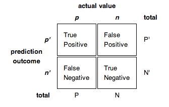
![](images/rocdiagram.png)

``` r
roc <- calculate_roc(heart_train$prediction, 
					 heart_train$num == 1)
summary(roc)
```

```
## AUC = 0.908
## Cost of false-positive = 1
## Cost of false-negative = 1
## Threshold with minimum cost = 0.606
```

]

---
# ROC Curve

.center[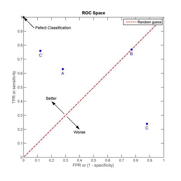
![](images/ROCspace.png)
]

---
# ROC Curve

``` r
plot(roc, curve = 'accuracy')
```

---
# ROC Curve

``` r
plot(roc, curve = 'cost')
```

---
# ROC Curve (false-negative up-weighted)

.pull-left[

``` r
roc2 <- calculate_roc(
	heart_train$prediction, 
	heart_train$num == 1,
	cost_of_fn = 2,
	cost_of_fp = 1)
summary(roc2)
```

```
## AUC = 0.908
## Cost of false-positive = 1
## Cost of false-negative = 2
## Threshold with minimum cost = 0.525
```
]
.pull-right[

``` r
plot(roc2, curve = 'cost')
```

<img src="07-Trees_files/figure-html/unnamed-chunk-25-1.png" alt="" style="display: block; margin: auto;" />
]

---
class: font90
# Caution on Interpreting Accuracy

- [Loh, Sooo, and Zing](http://cs229.stanford.edu/proj2016/report/LohSooXing-PredictingSexualOrientationBasedOnFacebookStatusUpdates-report.pdf) (2016) predicted sexual orientation based on Facebook Status.

- They reported model accuracies of approximately 90% using SVM, logistic regression and/or random forest methods.

- [Gallup](https://news.gallup.com/poll/234863/estimate-lgbt-population-rises.aspx) (2018) poll estimates that 4.5% of the Americal population identifies as LGBTG+.

- *My proposed model:* I predict all Americans are heterosexual.

- The accuracy of my model is 95.5%, or *5.5% better than Facebook's model!*

- Predicting "rare" events (i.e. when the proportion of one of the two outcomes large) is difficult and requires independent (predictor) variables that strongly associated with the dependent (outcome) variable.

---
# Fitted Values Revisited

What happens when the ratio of true-to-false increases (i.e. want to predict "rare" events)?

Let's simulate a dataset where the ratio of true-to-false is 10-to-1. We can also define the distribution of the dependent variable. Here, there is moderate separation in the distributions.

``` r
test.df2 <- getSimulatedData(
	treat.mean=.6, control.mean=.4)
```

The `multilevelPSA::psrange` function will sample with varying ratios from 1:10 to 1:1. It takes multiple samples and averages the ranges and distributions of the fitted values from logistic regression.

``` r
psranges2 <- psrange(test.df2, test.df2$treat, treat ~ .,
					 samples=seq(100,1000,by=100), nboot=20)
```

---
# Fitted Values Revisited (cont.)

``` r
plot(psranges2)
```

---
class: left, font140
# One Minute Paper

.pull-left[
1. What was the most important thing you learned during this class?
2. What important question remains unanswered for you?
]
.pull-right[
<img src="07-Trees_files/figure-html/unnamed-chunk-30-1.png" alt="" style="display: block; margin: auto;" />
.center[.font50[[Scan the QR code or click here to  
complete the One Minute Paper](https://docs.google.com/forms/d/e/1FAIpQLSdkRhGhJpsgc_0LxAmJpemlf7bni8Qs0ZUmovOVvHaOwOQyhA/viewform?usp=pp_url&entry.603740146=Fall2026&entry.1577539103=Tree%20Based%20Methods&entry.1379071784=IS382)]]
]